Designing Neural Networks in Mathematica

2021-05-15 7 min read Mathematics, Programming

Introduction

Wolfram Mathematica provides a comfortable machine learning framework to play around with. I can’t say how useful it is for real world problems because I’m just playing with it on my kindergarten projects, but I enjoyed working with it so far. There are a few things that I noted, though:

The documentation lists many of the functions as experimental. I assume this means that they might change in future releases.
I didn’t encounter any bugs or other issues, however the documentation is not always as clear as I am used from a software like Mathematica (Mathematica and Matlab have both some of the best documentation I have ever seen). I had to go through several manual pages and tutorials to get all the things together to get the code in this article running.
The built-in functionality to retrieve data is not 100% consistent. You can train on the fashion MNIST data set by entering its name, but you can’t explicitly retrieve the dataset.

LeNet and MNIST

There’s a tutorial in the Mathematica documentation that we will loosely follow. The goal is to set up a LeNet neural network and train it on the MNIST data set of handwritten digits.

Step 1: Getting the Data

The simplest way to get labelled data into our notebooks is via the commands:

trainingData = ResourceData["MNIST", "TrainingData"];
testData = ResourceData["MNIST", "TestData"];

The function ResourceData gives us the content of a ResourceObject. There are countless ResourceObjects of all kinds that you can query in Mathematica. I must admit that I am not quite sure how the Resource* functions relate to the ExampleData command that seems to fulfil a similar purpose and has been around for a much longer time. Also, it seems that “MNIST” is available, but “FashionMNIST” is not. Which is strange, because you can easily train on the latter by entering its name (see below).

Once we have the data, we must set up a way to encode the data (our input will be lots of small images) and to specify the output that we expect. In this case:

The input will be grayscale images of size 28×28
The output shall be a single digit number ranging from 0 to 9.

Again there are functions for this: NetEncoder and NetDecoder. They take care of the internal representation of the data and ensure that input and output works flawlessly.

mnistEncoder = NetEncoder[{
   "Image", {28, 28},
   "ColorSpace" -> "Grayscale"
}];
mnistDecoder = NetDecoder[{
   "Class", Range[0, 9]
}];

Step 2: Setting up the Network

The command NetChain specifies a neural network by concatenating the provided list of layers. Implementing LeNet is thus done as follows.

uninitializedNet = NetChain[{
   ConvolutionLayer[20, 5],
   ElementwiseLayer[Ramp],
   PoolingLayer[2, 2],
   ConvolutionLayer[50, 5],
   ElementwiseLayer[Ramp],
   PoolingLayer[2, 2],
   FlattenLayer[],
   LinearLayer[500],
   ElementwiseLayer[Ramp],
   LinearLayer[10],
   SoftmaxLayer[]
   },
  "Input" -> mnistEncoder,
  "Output" -> mnistDecoder
];

Note that the previous command only creates the neural network. The learnable parameters do not have any initial values yet. We must explicitly initialize them via:

initializedNet = NetInitialize[uninitializedNet];

In this example the convolution and linear layers have learnable parameters that need to be tuned. Note that the network would be usable at this point. The parameters have been given randomized values. The obtained results wouldn’t be great.

Step 3: Training the Network

In order to train our network we must provide a way to evaluate it. So far, our network accepts a single input (an image) and returns a single number (the estimated digit). If we want to train our network, we must be able to feed it the input image together with its known label. To this end we must convert it to a graph and add a cross entropy layer as loss estimate.

trainingNet = NetGraph[
   <|
    "MyNet" -> initializedNet,
    "loss" -> CrossEntropyLossLayer["Index"]
   |>,
   {
    NetPort["Input"] -> "MyNet" -> NetPort["loss", "Input"],
    NetPort["Target"] -> NetPort["loss", "Target"]
   }
];

In the code above, the first part specifies the available networks and layers. The second part specifies how everything is connected. Besides our network (now named “MyNet”) we have added a layer “loss”, which is given by a cross entropy layer. Input data goes to the “Input” port of our network, flows through “MyNet” and into the “Input” port of the “loss” layer. The data labels go to the “Target” port of our network and flow directly to the “Target” port of our “loss” layer.

In order to train our network we must specify some training data and some validation data.

trainAssoc = <|
   "Input" -> Keys[trainingData],
   "Target" -> Values[trainingData] + 1
|>;
testAssoc = <|
   "Input" -> Keys[testData],
   "Target" -> Values[testData] + 1
|>;

The +1 is necessary because our labels are digits going from 0 to 9, our loss function however works with indices of a list of 10 probabilities. Since array indices are 1 based in Mathematica, we must add 1 to each value. Training is now straightforward.

results = NetTrain[
   trainingNet,
   trainAssoc,
   All,
   ValidationSet -> testAssoc,
   MaxTrainingRounds -> 5
];

As a final step we remove the cross entropy layer and reattach the original input/output encoders and decoders.

trainedNet = NetExtract[results["TrainedNet"], "MyNet"];
trainedNet = NetReplacePart[
   trainedNet,
   {"Input" -> mnistEncoder,
    "Output" -> mnistDecoder}
];

Step 4: Evaluating the Network

The training already provides a lot of information. Even more information can programmatically be queried as well.

measurements = ClassifierMeasurements[trainedNet, testData];
measurements["Accuracy"]

NetMeasurements[trainedNet, testData, "ConfusionMatrixPlot"]

Here we ask for the accuracy of the network and plot its confusion matrix. The accuracy should be somewhere around 0.99.

Appendix: Predefined Networks and other Implementations

Mathematica offers a set of predefined neural networks. They can be used via the command NetModel. We could simply have taken the pretrained network if we were only interested in the network.

trainedNet2 = NetModel["LeNet Trained on MNIST Data"];
measurements = ClassifierMeasurements[trainedNet2, testData];
measurements["Accuracy"]
NetMeasurements[trainedNet, testData, "ConfusionMatrixPlot"]

A somewhat longer and more explicit version would be. Here we leave the creation of the graph and the addition of the loss function to the NetTrain method.

uninitializedNet = NetChain[{
    ConvolutionLayer[20, 5],
    ElementwiseLayer[Ramp],
    PoolingLayer[2, 2],
    ConvolutionLayer[50, 5],
    ElementwiseLayer[Ramp],
    PoolingLayer[2, 2],
    FlattenLayer[],
    LinearLayer[500],
    ElementwiseLayer[Ramp],
    LinearLayer[10],
    SoftmaxLayer[]
    },
   "Input" -> mnistEncoder,
   "Output" -> mnistDecoder
];
trainedNet3 = NetTrain[
  uninitializedNet,
  "MNIST",
  MaxTrainingRounds -> 5,
  TargetDevice -> "GPU",
  LossFunction -> CrossEntropyLossLayer["Index"]
  ]
measurements = ClassifierMeasurements[trainedNet3, testData];
measurements["Accuracy"]
NetMeasurements[trainedNet3, testData, "ConfusionMatrixPlot"]

Testing my own handwriting.

I don’t consider my handwriting to be illegible, thus I was expecting a near perfect recognition of my own handwriting. Apparently my trained network had an accuracy of 0.9925 and yet it couldn’t decipher 3 of my own digits. It failed for the digits 0 (recognized as 9), 7 (recognized as 5), and 9 (recognized as 5) depicted below.

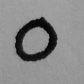
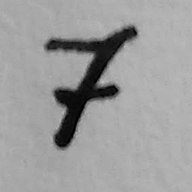
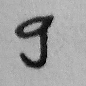
All digits are available here. The images are 280×280, so you have to resize them to 28×28. Binarizing the image didn’t change anything on the result for me.

Final thoughts

The code in this article provides an excellent start to play around with neural networks. Exchanging layers and investigating the impact is straightforward. Exchanging the dataset is also not too hard. The named dataset in the NetTrain call for trainedNet3 can for example be replaced by “FashionMNIST”.

trainedNet3 = NetTrain[
  NetChain[{
    ConvolutionLayer[20, 5], ElementwiseLayer[Ramp], 
    PoolingLayer[2, 2], ConvolutionLayer[50, 5], 
    ElementwiseLayer[Ramp], PoolingLayer[2, 2], FlattenLayer[], 
    LinearLayer[500], ElementwiseLayer[Ramp], LinearLayer[10], 
    SoftmaxLayer[]}, "Input" -> mnistEncoder, 
   "Output" -> mnistDecoder],
  "FashionMNIST",
  MaxTrainingRounds -> 5,
  TargetDevice -> "GPU",
  LossFunction -> CrossEntropyLossLayer["Index"]
  ]
NetMeasurements[trainedNet3, "FashionMNIST", "ConfusionMatrixPlot"]

Other datasets, such as “CIFAR-100” can easily be used as well since they can be loaded with ResourceData. To use them we would have to adapt the encoders and decoders, though.

References

[1] Wikipedia contributors, “LeNet,” Wikipedia, The Free Encyclopedia, URL (accessed May 15, 2021).
[2] Wikipedia contributors, “MNIST database,” Wikipedia, The Free Encyclopedia, URL (accessed May 15, 2021).
Notes
All code sample in this article have been evaluated with Wolfram Mathematica 12.2.0.0